Using maxcovr
Nicholas Tierney
2025-04-30
Source:vignettes/intro_to_maxcovr.Rmd
intro_to_maxcovr.Rmdmaxcovr provides tools to make it easy to solve the “maximum covering location problem”, a binary optimisation problem described by Church.
maxcovr aims to provide researchers and analysts with an
easy to user, fast, accurate and (eventually) extensible implementation
of Church’s maximal covering location problem, while adhering as best as
it can to tidyverse
principles.
This vignette aims to get users started with using maxcovr. In this vignette you will learn about:
- The motivation behind
maxcovr - How to assess current coverage of facilities
- How to maximise coverage using some new proposed facilities
- Explore results of the new locations
- How to explore the new locations proposed
Other vignettes provided in the package include:
- “Cross Validation with maxcovr”, which explains how to perform and interpret cross validation results in a maximum covering location framework
- “Performing the maximal coverage relocation problem”
The moviation: Why maxcovr
maxcovr was created to make it easy for a non expert to
correctly solve the maximum covering location problem. This problem is
beginning to be applied in problems in AED placement, but
has been applied in many different areas. Many
implementations in papers apply commercial software such as AMPL,
Gurobi, or CPLEX. Additionally, the code that they use in the paper to
implement the optimisation is not provided, and has to be requested. As
a result, these analyses are more difficult to implement, and more
difficult to reproduce.
maxcovr was created to address these shortcomings,
using:
- R, a free and open source language
- Open source solvers, lpSolve, and glpk, that can be used on Linux, Windows, and OSX.
- Real-world, open source example data.
- Tidyverse principles to design it for humans make it easy to use, code, and extend.
This means results are easy to implement, reproduce, and extend.
The problem
Consider the toy example where we want to place crime surveillance
towers to detect crime. We have two datasets, york, and
york_crime:
-
yorkcontains listed building GPS locations in the city of York, provided by the city of york -
york_crimecontains a set of crime data from theukpolicepackage, containing crime data from September 2016.
We already have a few surveillance towers built, which are placed on
top of the listed buildings with a grade of I. We will call this dataset
york_existing, and the remaining building locations
york_proposed. Here, york_existing is the
currently locations of facilities, and york_proposed is the
potential facility locations.
##
## Attaching package: 'dplyr'
## The following objects are masked from 'package:stats':
##
## filter, lag## The following objects are masked from 'package:base':
##
## intersect, setdiff, setequal, union
# subset to be the places with towers built on them.
york_existing <- york %>% filter(grade == "I")

york_proposed <- york %>% filter(grade != "I")
We are interested in placing surveillance towers so that they are within 100m of the largest number of crimes. We are going to use the crime data that we have to help us choose ideal locations to place towers.
This can be illustrated with the following graphic, where the red circles indicate the current coverage of the building locations, so those blue crimes within the circles are within the coverage.
## Assuming "long" and "lat" are longitude and latitude, respectively
## Assuming "long" and "lat" are longitude and latitude, respectively
Visually, the coverage looks OK, but to get a better estimate, we can
verify the coverage using the nearest() function.
nearest() takes two dataframes and returns the nearest
lat/long coords from the first dataframe to the second dataframe, along
with the distances between them and the appropriate columns from the
building dataframe. You can think of reading this as “What is the
nearest (nearest_df) to (to_df)”.
## # A tibble: 6 × 22
##   to_id nearest_id distance category          persistent_id date  lat_to long_to
##   <dbl>      <dbl>    <dbl> <chr>             <chr>         <chr>  <dbl>   <dbl>
## 1     1       1787   18.2   anti-social-beha… 62299914865f… 2016…   54.0   -1.08
## 2     2        794  512.    anti-social-beha… 4e34f53d247f… 2016…   54.0   -1.12
## 3     3        350    0.993 anti-social-beha… 2a0062f3dfac… 2016…   54.0   -1.08
## 4     4        327   20.5   anti-social-beha… eb53e09ae46a… 2016…   54.0   -1.09
## 5     5       1860  135.    anti-social-beha… 6139f131b724… 2016…   54.0   -1.08
## 6     6        404   22.8   anti-social-beha… d8de26d5af47… 2016…   54.0   -1.08
## # ℹ 14 more variables: street_id <chr>, street_name <chr>, context <chr>,
## #   id <chr>, location_type <chr>, location_subtype <chr>,
## #   outcome_status <chr>, long_nearest <dbl>, lat_nearest <dbl>,
## #   object_id <int>, desig_id <chr>, pref_ref <int>, name <chr>, grade <chr>
Note that
maxcovrrecords the positions of locations must be named “lat” and “long” for latitude and longitude, respectively.
The dataframe dat_dist contains the nearest proposed
facility to each crime. This means that we have a dataframe that
contains “to_id” - the ID number (labelled from 1 to the number of rows
in the to dataset), “nearest_id” describes the row numer of “nearest_df”
that corresponds to the row location of that data.frame. We also have
the rest of the columns of york_crime. These are returned
to make it easy to do other data manipulation / exploration tasks, if
you wish.
You can instead return a dataframe which has every building in the rows, and the nearest crime to the building, by simply changing the order.
## # A tibble: 6 × 22
##   to_id nearest_id distance long_to lat_to object_id desig_id pref_ref name
##   <dbl>      <dbl>    <dbl>   <dbl>  <dbl>     <int> <chr>       <int> <chr>
## 1     1         33     36.0   -1.09   54.0      6144 DYO1195    463280 GUILDHAL…
## 2     2        183     35.8   -1.09   54.0      6142 DYO1373    462942 BOOTHAM …
## 3     3        503     95.3   -1.08   54.0      3463 DYO365     464845 THE NORM…
## 4     4        273     44.3   -1.08   54.0      3461 DYO583     464427 CHURCH O…
## 5     5        908     26.5   -1.08   54.0      3460 DYO916     463764 CUMBERLA…
## 6     6        495    326.    -1.13   54.0      3450 DYO1525    328614 CHURCH O…
## # ℹ 13 more variables: grade <chr>, category <chr>, persistent_id <chr>,
## #   date <chr>, lat_nearest <dbl>, long_nearest <dbl>, street_id <chr>,
## #   street_name <chr>, context <chr>, id <chr>, location_type <chr>,
## #   location_subtype <chr>, outcome_status <chr>
To evaluate the coverage we use coverage, specifying the
distance cutoff in distance_cutoff to be 100m.
coverage(york_proposed,
         york_crime,
         distance_cutoff = 100)
## # A tibble: 1 × 7
## distance_within n_cov n_not_cov prop_cov prop_not_cov dist_avg dist_sd
## <dbl> <int> <int> <dbl> <dbl> <dbl> <dbl>
## 1 100 685 1129 0.378 0.622 355. 422.This contains useful summary information:
- distance_within - this is the distance used to determine coverae
- n_cov - this is the number of events that are covered
- n_not_cov - the number of events not covered
- pct_cov - the proportion of events covered
- pct_not_cov - the proportion of events not covered
- dist_avg - the average distance from the rows to the nearest facility or user
- dist_avg - the standard deviation of the distance from the rows to the nearest facility or user.
This tells us that out of all the crime, 37.76% of it is within 100m, 339 crimes are covered, but the mean distance to the surveillance camera is 1400m.
using max_coverage
Knowing this information, you might be interested in improving this
coverage. To do so we can use the max_coverage
function.
This function takes 5 arguments:
- existing_facility = the facilities currently installed
- proposed_facility = the facilities proposed to install
- user = the users that you want to maximise coverage over
- n_added = the number of new facilities that you can install
- distance_cutoff = the distance that we consider coverage to be within.
Similar to using nearest - the data frames for
existing_facility, proposed_facility, and user need to contain columns
of latitude and longitude, and they must be named “lat”, and “long”,
respectively. These are used to calculate the distance.
# mc_20 <- max_coverage(A = dat_dist_indic,
mc_20 <- max_coverage(existing_facility = york_existing,
                      proposed_facility = york_proposed,
                      user = york_crime,
                      n_added = 20,
                      distance_cutoff = 100)
We can look at a quick summary of the model with summary
summary(mc_20)##
## -------------------------------------------
## Model Fit: maxcovr fixed location model
## -------------------------------------------
## Distance Cutoff: 100m
## Facilities:
## Added: 20
## Coverage (Previous):
## # Users: 540 (339)
## Proportion: 0.2977 (0.1869)
## Distance (m) to Facility (Previous):
## Avg: 886 (1400)
## SD: 986 (1597)
## -------------------------------------------Here this tells us useful information about the distance cutoff, the number of facilities added, and the number of users covered, and previousl, and the proportion of events covered.
To get this information out we can use the information in each of the
columns below. The information each of these is a list, which might seem
strange, but it becomes very useful when you are assessing different
levels of n_added. We will go into more detail for this
soon.
Firstly, we have the data input into n_added and
distance_cutoff - the same information that we entered.
mc_20$n_added[[1]]## [1] 20
mc_20$distance_cutoff[[1]]## [1] 100We can then get summary information about the model coverage. We can
first get the existing, or previous coverage with
existing_coverage
mc_20$existing_coverage[[1]]## # A tibble: 1 × 8
## n_added distance_within n_cov pct_cov n_not_cov pct_not_cov dist_avg dist_sd
## <dbl> <dbl> <int> <dbl> <int> <dbl> <dbl> <dbl>
## 1 0 100 339 0.187 1475 0.813 1400. 1597.This provides us with the information that we saw previously with
summarise_coverage.
We can then get the information of the coverage from the model with
the added additional AEDs with model_coverage.
mc_20$model_coverage[[1]]## # A tibble: 1 × 8
## n_added distance_within n_cov pct_cov n_not_cov pct_not_cov dist_avg dist_sd
## <dbl> <dbl> <int> <dbl> <int> <dbl> <dbl> <dbl>
## 1 20 100 540 0.298 1274 0.702 886. 986.We can then get both pieces of information from
summary
mc_20$summary[[1]]## # A tibble: 2 × 8
## n_added distance_within n_cov pct_cov n_not_cov pct_not_cov dist_avg dist_sd
## <dbl> <dbl> <int> <dbl> <int> <dbl> <dbl> <dbl>
## 1 0 100 339 0.187 1475 0.813 1400. 1597.
## 2 20 100 540 0.298 1274 0.702 886. 986.You can drill deeper, and get more information about the facilities
using facility_selected, which returns facilities selected
from the proposed_facility data.
mc_20$facility_selected[[1]]## # A tibble: 20 × 7
## long lat object_id desig_id pref_ref name grade
## <dbl> <dbl> <int> <chr> <int> <chr> <chr>
## 1 -1.09 54.0 5978 DYO1383 462917 NA II
## 2 -1.08 54.0 5909 DYO1297 463072 NA II
## 3 -1.08 54.0 5872 DYO1244 463186 NA II
## 4 -1.08 54.0 5847 DYO1216 463242 NA II
## 5 -1.12 54.0 5759 DYO1108 463434 FORMER JUNIOR SCHOOL BUILDING … II
## 6 -1.08 54.0 5748 DYO1096 463469 NA II
## 7 -1.08 54.0 5745 DYO1093 463465 NA II
## 8 -1.08 54.0 5739 DYO1086 463457 CHURCH OF ST GEORGE AND ATTACH… II
## 9 -1.10 54.0 5642 DYO960 463695 NA II
## 10 -1.09 53.9 5606 DYO920 463771 PRESS STAND AT YORK RACECOURSE II
## 11 -1.06 54.0 5592 DYO903 463788 NA II
## 12 -1.07 54.0 5588 DYO899 463782 NA II
## 13 -1.08 54.0 5529 DYO829 463938 CHURCH OF ST THOMAS II
## 14 -1.08 54.0 5454 DYO705 464133 NUMBERS 45-51 (ODD) AND ATTACH… II
## 15 -1.03 54.0 5373 DYO1644 NA War Memorial II
## 16 -1.12 54.0 5349 DYO572 464451 POPPLETON ROAD SCHOOL II
## 17 -1.08 54.0 5328 DYO544 464508 WOODS MILL II
## 18 -1.00 54.0 3215 DYO1581 491367 STOCKTON GRANGE AND ATTACHED O… II
## 19 -1.08 54.0 3213 DYO1580 490659 NEW CHAPEL AT ST JOHN'S COLLEGE II
## 20 -1.08 54.0 4803 DYO1734 NA The Swan Public House IIWe can then get information about the users with
augmented_users
mc_20$augmented_users[[1]]## # A tibble: 1,814 × 19
## to_id nearest_id distance user_id category persistent_id date lat_to long_to
## <dbl> <dbl> <dbl> <int> <chr> <chr> <chr> <dbl> <dbl>
## 1 1 3 84.3 1 anti-so… 62299914865f… 2016… 54.0 -1.08
## 2 2 16 512. 2 anti-so… 4e34f53d247f… 2016… 54.0 -1.12
## 3 3 3 65.2 3 anti-so… 2a0062f3dfac… 2016… 54.0 -1.08
## 4 4 31 286. 4 anti-so… eb53e09ae46a… 2016… 54.0 -1.09
## 5 5 20 231. 5 anti-so… 6139f131b724… 2016… 54.0 -1.08
## 6 6 8 22.8 6 anti-so… d8de26d5af47… 2016… 54.0 -1.08
## 7 7 22 2136. 7 anti-so… 5b742b1cb918… 2016… 54.0 -1.09
## 8 8 26 2329. 8 anti-so… d2112b4fd0a0… 2016… 54.0 -1.11
## 9 9 49 37.4 9 anti-so… 30bf5bfa97c5… 2016… 54.0 -1.09
## 10 10 5 3150. 10 anti-so… d75bbe6c18bf… 2016… 54.0 -1.17
## # ℹ 1,804 more rows
## # ℹ 10 more variables: street_id <chr>, street_name <chr>, context <chr>,
## # id <chr>, location_type <chr>, location_subtype <chr>,
## # outcome_status <chr>, lat_nearest <dbl>, long_nearest <dbl>, type <chr>This returns the dataframe of users, with the distance to their
nearest AED, and at the end, provides information about the
type of AED that is used.
Now try and run the code for n_added = 40, and call it “mc_40”
Interpreting results
We can assess what happens if we add 100 facilities.
mc_100 <- max_coverage(existing_facility = york_existing,
                      proposed_facility = york_proposed,
                      user = york_crime,
                      n_added = 100,
                      distance_cutoff = 100)
summary(mc_100)##
## -------------------------------------------
## Model Fit: maxcovr fixed location model
## -------------------------------------------
## Distance Cutoff: 100m
## Facilities:
## Added: 100
## Coverage (Previous):
## # Users: 693 (339)
## Proportion: 0.382 (0.1869)
## Distance (m) to Facility (Previous):
## Avg: 555 (1400)
## SD: 696 (1597)
## -------------------------------------------So then, if we want to add information to discover the differences
between 20 and 100, we can bind these two pieces together using
bind_rows.
mc_20_100 <- bind_rows(mc_20, mc_100)We can then look at the summary row, and expand the information out
here using tidyr::unnest()
## Warning: `cols` is now required when using `unnest()`.
## ℹ Please use `cols = c(summary)`.
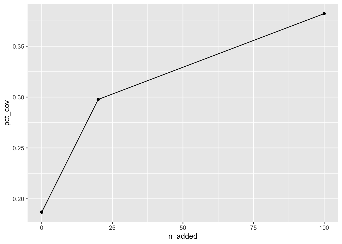
mc_20_100_sum## # A tibble: 4 × 8
## n_added distance_within n_cov pct_cov n_not_cov pct_not_cov dist_avg dist_sd
## <dbl> <dbl> <int> <dbl> <int> <dbl> <dbl> <dbl>
## 1 0 100 339 0.187 1475 0.813 1400. 1597.
## 2 20 100 540 0.298 1274 0.702 886. 986.
## 3 0 100 339 0.187 1475 0.813 1400. 1597.
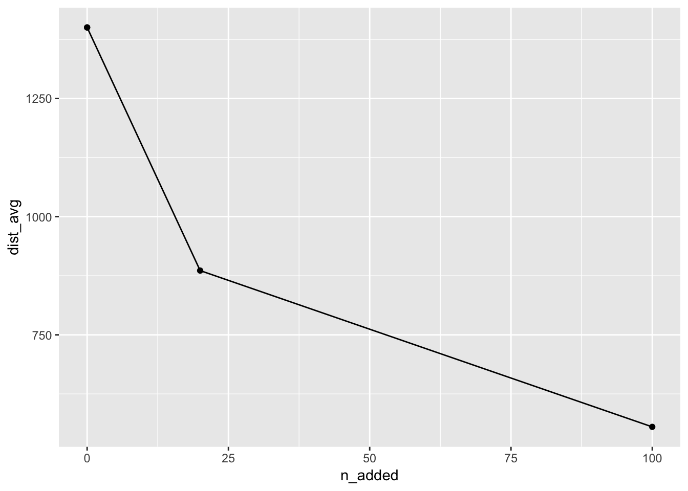
## 4 100 100 693 0.382 1121 0.618 555. 696.This information can then be plotted, for example, like so:
You can then produce a plot of the average distances.
If you would like to calculate your own summaries on the distances, I would recommend something like:
mc_20$augmented_users[[1]] %>%
    summarise(mean_dist = mean(distance),
              sd_dist = sd(distance),
              median_dist = median(distance),
              lower_975_dist = quantile(distance, probs = 0.025),
              upper_975_dist = quantile(distance, probs = 0.975))
## # A tibble: 1 × 5
## mean_dist sd_dist median_dist lower_975_dist upper_975_dist
## <dbl> <dbl> <dbl> <dbl> <dbl>
## 1 886. 986. 613. 17.1 3526.You can then package this up in a function and apply it to all rows
my_dist_summary <-  function(data){
    data %>%
    summarise(mean_dist = mean(distance),
              sd_dist = sd(distance),
              median_dist = median(distance),
              lower_975_dist = quantile(distance, probs = 0.025),
              upper_975_dist = quantile(distance, probs = 0.975))
}
This can then be used to create a new column with
purrr::map().
mc_20_100 %>%
    mutate(new_summary = purrr::map(augmented_users,
                                    my_dist_summary)) %>%
    select(new_summary) %>%
    tidyr::unnest()
## Warning: `cols` is now required when using `unnest()`.
## ℹ Please use `cols = c(new_summary)`.## # A tibble: 2 × 5
## mean_dist sd_dist median_dist lower_975_dist upper_975_dist
## <dbl> <dbl> <dbl> <dbl> <dbl>
## 1 886. 986. 613. 17.1 3526.
## 2 555. 696. 307. 16.2 2277.Other graphics options
You might be interested in plotting the existing users, the proposed facilities, and the coverage.
You can plot the existing facilities with leaflet.
york_existing %>%
    leaflet() %>%
    addTiles() %>%
    addCircles(color = "steelblue") %>%
    setView(lng = median(york_existing$long),
            lat = median(york_existing$lat),
            zoom = 12)
## Assuming "long" and "lat" are longitude and latitude, respectivelyYou might want to then add the user information to this plot. You can add new circles based on new datasets, and then change the colour, so that they are visible.
leaflet() %>%
    addCircles(data = york_crime,
               color = "steelblue") %>%
    addCircles(data = york_existing,
               color = "coral") %>%
    addTiles() %>%
    setView(lng = median(york$long),
            lat = median(york$lat),
            zoom = 15)
## Assuming "long" and "lat" are longitude and latitude, respectively
## Assuming "long" and "lat" are longitude and latitude, respectivelyWith leaflet you can also specify the radius in metres of the circles. This means that we can set the radius of the circles to be 100, and this is 100m.
leaflet() %>%
addCircles(data = york_crime,
color = "steelblue") %>%
addCircles(data = york_existing,
radius = 100,
color = "coral") %>%
addTiles() %>%
setView(lng = median(york$long),
lat = median(york$lat),
zoom = 15)## Assuming "long" and "lat" are longitude and latitude, respectively
## Assuming "long" and "lat" are longitude and latitude, respectivelyto make this a bit clearer we can remove the fill
(fill = FALSE), and also change the map that is used with
addProviderTiles("CartoDB.Positron").
leaflet() %>%
addCircles(data = york_crime,
color = "steelblue") %>%
addCircles(data = york_existing,
radius = 100,
fill = FALSE,
color = "coral",
weight = 3,
dashArray = "1,5") %>%
addProviderTiles("CartoDB.Positron") %>%
setView(lng = median(york$long),
lat = median(york$lat),
zoom = 15)## Assuming "long" and "lat" are longitude and latitude, respectively
## Assuming "long" and "lat" are longitude and latitude, respectivelyApplying this to the coverage data
So using this knowledge, we can visualise:
- crime (
york_crime) - existing facilities (
york_existing) - newly placed facilities
(
mc_20$facility_selected[[1]])
leaflet() %>%
addCircles(data = york_crime,
color = "steelblue") %>%
addCircles(data = york_existing,
radius = 100,
fill = FALSE,
weight = 3,
color = "coral",
dashArray = "1,5") %>%
addCircles(data = mc_20$facility_selected[[1]],
radius = 100,
fill = FALSE,
weight = 3,
color = "green",
dashArray = "1,5") %>%
addProviderTiles("CartoDB.Positron") %>%
setView(lng = median(york$long),
lat = median(york$lat),
zoom = 15)## Assuming "long" and "lat" are longitude and latitude, respectively
## Assuming "long" and "lat" are longitude and latitude, respectively
## Assuming "long" and "lat" are longitude and latitude, respectively